From Gauss's mean error to Yule's standard error
To fully appreciate the math we are about to discuss, we must first rewind our clock to 1911.

1911 is an important year for students of statistics. For one, the world's first statistics department was founded by Karl Pearson (1857 – 1936) in UCL. And two, the world's first statistics textbook was published by Udny Yule (1871 – 1951).
And the following is what Yule has to say about standard deviation in his textbook (p. 134):
The standard deviation is the square root of the arithmetic mean of the squares of all deviations, deviations being measured from the arithmetic mean of the observations. If the standard deviation be denoted by \(\sigma\), and a deviation from the arithmetic mean by \(x\), as in the last chapter, then the standard deviation is given by the equation \(\sigma^2=\frac{1}{N}\sum x^2\). To square all the deviations may seem at first sight an artificial procedure, but it must be remembered that it would be useless to take the mere sum of the deviations, in order to obtain some quantity that shall vary with the dispersion it is necessary to average the deviations by a process that treats them as if they were all of the same sign, and squaring is the simplest process for eliminating signs which leads to results of algebraic convenience.
However, Yule was not the originator of the term, for he learnt it first hand from his boss, who must have coined the word sometime before 1894. In the second part of his 1894 paper, Pearson wrote (p. 75):
. . . in the case of a frequency-curve whose components are two normal curves, the complete solution depends in the method adopted in finding the roots of a numerical equation of the ninth order. It is possible that a simpler solution may be found, but the method adopted has only been chosen after many trials and failures. Clearly each component normal curve has three variables: (i) the position of its axis, (ii) its “standard-deviation" (Gauß's “Mean Error", Airy's “Error of Mean Square"), and (iii) its area . . .Apparently Pearson was aware that his standard deviation is equivalent to Airy's error of mean square. And in general Airy's error of mean of the \(n\)-th order is, when raised to the \(n\)-th power, equivalent to Pearson's moment of the \(n\)-th order around zero: $$ \begin{align} \underbrace{\textrm{mean error/error of mean}}_\textrm{of $n$-th order (to the $n$-th power)} &= (\epsilon_n)^n \\ &= \frac{\displaystyle \int\limits_x x^n\,df}{\displaystyle \int\limits_x\,df}\\ &= \underbrace{\mu_n'}_{\textrm{$n$-th moment}} \end{align} $$
For instance, when Airy applied the formula to his error frequency element \(df = \frac{A}{c\sqrt{\pi}}e^{-(x/c)^2}\,dx\), \(x \in [0,+\infty)\) (the constant \(c\) in the element was termed modulus by Airy), he obtained:
\begin{align} \underbrace{\textrm{mean error} = \epsilon_1}_\textrm{linear mean} &= \tfrac{c}{\sqrt{\pi}} = 0.564c\\ \underbrace{\textrm{error of mean square} = \epsilon_2}_\textrm{quadratic mean (or root-mean-square)} &= \tfrac{c}{\sqrt{2}} = 0.707c\\ \qquad \qquad & \qquad \vdots \qquad\\ & \textrm{and in general}\\ \qquad \qquad & \qquad \vdots \qquad\\ \epsilon_n &= c\left(\tfrac{\Gamma\left(\tfrac{n+1}{2}\right)}{\sqrt{\pi}}\right)^{\frac{1}{n}} \end{align}Besides mean error and error of mean square, the term probable error \(\epsilon_p\) was also mentioned by Airy in his book.
It has however been customary to make use of a different number, called the Probable Error. It is not meant by this term that the number used is a more probable value of error than any other value, but that, when the positive sign is attached to it, the number of positive errors larger than the value is about as great as the number of positive errors smaller than that value . . .
which is essentially the median error: $$\int_0^{\epsilon_p} \,df = \int_{\epsilon_p}^\infty \,df$$ $$\textrm{probable error} = \epsilon_p = 0.4769362762c$$ Now, to test your understanding on the subject, please try the following exam question:

From Airy's theory of error to Pearson's theory of variable: The need for a new term?
There are two reasons. The first reason is that since Pearson was extending the old theory of errors to a more general theory of variable for biological problems, he had to shift the center of origin of his frequency element to a non-zero value. Since his attention was on the biological measurements themselves (rather than the error associated with the measurements) and it is semantically incorrect for Pearson to repurpose Gauß's mean error and Airy's error of mean square for biological problems. $$\underbrace{\textrm{mittlere Fehler}}_\textrm{in everyday German} = \underbrace{\textrm{mean error}}_\textrm{in everyday English}$$ $$\underbrace{\textrm{mittlere Fehler}}_\textrm{$\epsilon_2$ by Gauß's definition (1821)} \neq \underbrace{\textrm{mean error}}_\textrm{$\epsilon_1$ by Airy's definition (1861)}$$
The second reason is that Gauß's der mittlere Fehler or errorem medium (literally mean error) is actually a quadratic mean error, and not Airy's mean error (which is a linear mean error).
$$\underbrace{\textrm{mittlere Fehler}}_\textrm{$\epsilon_2$ by Gauß's definition (1821)} = \underbrace{\textrm{error of mean square}}_\textrm{$\epsilon_2$ by Airy's definition (1861)}$$And Pearson must have reasoned to himself that the best way to solve the conundrum is to abandon both Gauß's mittlere Fehler and Airy's error of mean square. This problem was highlighted, for example, by William Chauvenet, in his astronomical manual (see p. 491):
. . . another error, very commonly employed in expressing the precision of observations, is that which has received the appellation of the mean error (der mittlere Fehler of the Germans), which is not to be confounded with the above mean of the errors. Its definition is, the error of the square of which is the mean of the squares of all the errors . . .
From Pearson's theory of variable to Yule's theory of sampling: Combining standard and error
Unfortunately, Yule soon encountered a problem and he had to reintroduce the word error in sampling-related statistics. And Yule decided that Pearson's standard and Airy's error must be blended to describe a common situation in sampling theory (Yule 1911, p. 262 - 263):
. . . the standard-deviation of simple sampling being the basis of all such work, it is convenient to refer to it by a shorter name. The observed proportions of \(A\)'s in given samples being regarded as differing by larger or smaller errors from the true proportion in a very large sample from the same material, the standard-deviation of simple sampling may be regarded as a measure of the magnitude of such errors, and may be called accordingly the standard error. . .
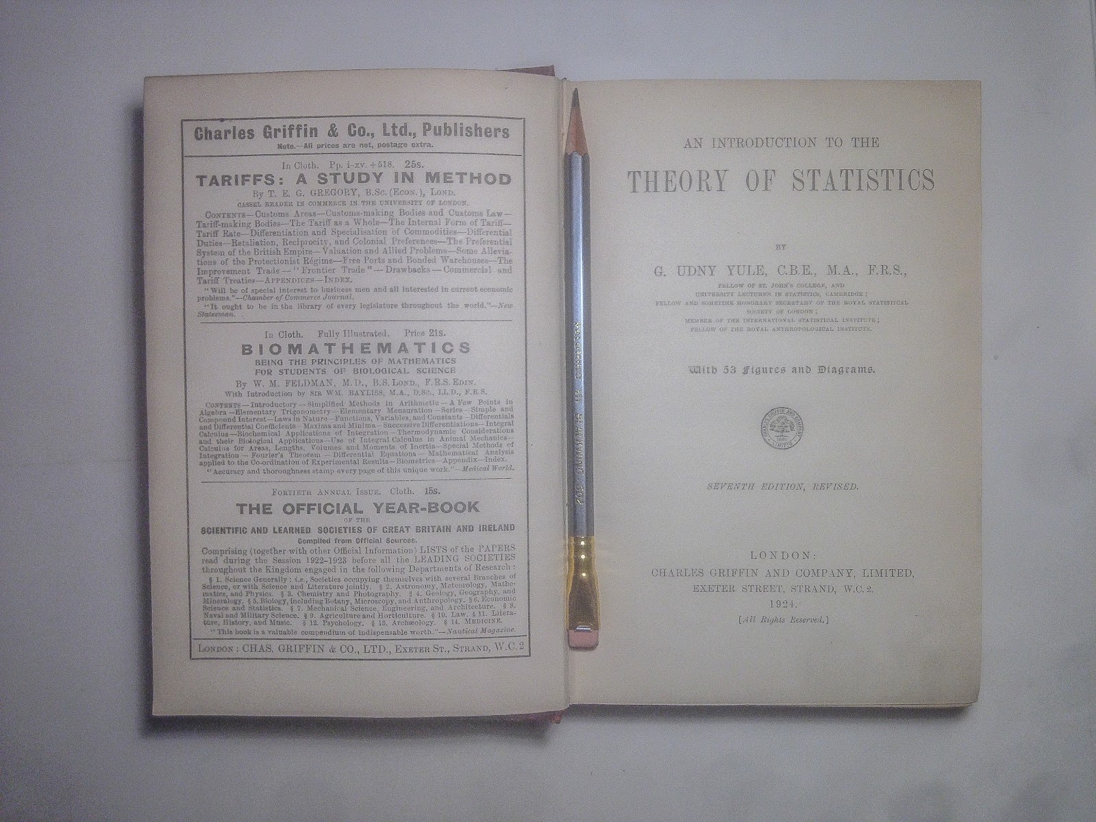
- G. U. Yule (1917) An introduction to the theory of statistics, 4th edition, Charles Griffin and Company, Ltd, London. Yule's book was first published in 1911. Pictured below is my own copy of the book (7th edition, 1924).
- see Karl Pearson (1893) Asymmetrical frequency curves. Nature 48, pp. 615 - 616; Karl Pearson (1894) Contributions to the mathematical theory of evolution. Philosophical Transactions of the Royal Society A 185, pp. 71 - 110. The paper was received on October 18, 1893 by the Royal Society and was read by Pearson's German colleague in UCL, Olaus Henrici. Note that Pearson's spelling is standard-deviation, with a dash in between the two words.
- George Biddell Airy (1875) On the algebraic and numerical theory of errors and the combination of observations, 2nd edition, Macmillan, London. The first edition of Airy's book was published in 1861.
- Airy's modulus \(c\) is equivalent to Gauß's \(1/h\) (in 1809), and Gauß's \(h\) (in 1821), for Gauß wrote his density function as \(\varphi\Delta = \frac{h}{\sqrt{\pi}}e^{-hh\Delta\Delta}\) in Theoria Motvs [see C. F. Gauß (1809) Theoria motvs corporvm coelestivm in sectionibvs conicis Solem ambientivm (Theory of the Motion of the Heavenly Bodies Moving about the Sun in Conic Sections)]. In 1821, however, Gauß inverted his \(h\) and wrote \(\displaystyle \varphi x = \frac{e^{-\frac{x}{h}\frac{x}{h}}}{h \sqrt{\pi}}\). [see C. F. Gauß (1821) Theoria combinationis observationum erroribus minimis obnoxiae (Theory of the combination of observations least subject to error)] In modern notation, Gauß's \(\varphi\)-function can be written as: \(\varphi(\Delta)=\frac{h}{\sqrt{\pi}}e^{-h^2 \Delta^2}\) or \(\varphi(x) = \frac{1}{h\sqrt{\pi}}e^{-x^2/h^2}\). When Fisher published his frequency curve paper [R. A. Fisher (1912) On an absolute criterion for fitting frequency curves, Messenger of Mathematics 41, pp. 155 - 160.], the 1809-notation was adopted: \(f = \frac{h}{\sqrt{\pi}}e^{-h^2(x-m)^2}\)
- Let \(df = \frac{\sigma^{n-2}}{\Sigma^{n-1}}e^{-\frac{n\sigma^2}{2\Sigma^2}}\,d\sigma\), then the mathematical expectation of \(\sigma\) can be written as
$$
\begin{align}\mathbf{E}(\sigma) &= \frac{\displaystyle \int_0^\infty x \,df}{\displaystyle \int_0^\infty df}\\
&=\Sigma \sqrt{\frac{2}{n}} \frac{\Gamma\left(\frac{n}{2}\right)}{\Gamma\left(\frac{n}{2}-\frac{1}{2}\right)}
\end{align}
$$
Also we can show that
$$
\begin{align} {\rm Var}(\sigma)
&= \mathbf{E}(\sigma^2) - \left(\mathbf{E}(\sigma)\right)^2\\
&= \Sigma^2 \left[1-\frac{1}{n}-\frac{2 \lambda^2 }{n} \right]
\end{align}
$$
where \(\lambda = \frac{\Gamma\left(\frac{n}{2}\right)}{\Gamma\left(\frac{n}{2}-\frac{1}{2}\right)}\), since
$$
\mathbf{E}(\sigma^2) = \frac{\displaystyle \int_0^\infty x^2 \,df}{\displaystyle \int_0^\infty df} =\left(1 - \tfrac{1}{n}\right)\Sigma^2
$$
From the reference distribution, we can also compute the following \(p\)-value:$$p=\frac{\displaystyle\int_{\sigma'}^\infty\,df}{\displaystyle \int_0^\infty\,df}=\frac{\Gamma\left(\frac{n}{2}-\frac{1}{2}, \frac{n}{2}\left(\frac{\sigma'}{\Sigma}\right)^2\right)}{\Gamma\left(\frac{n}{2}-\frac{1}{2}\right)}$$which is essentially the probability of getting sample standard deviation that is higher than \(\sigma'\). Furthermore, we can compute the following \(\alpha\)-confidence interval:$$\sigma_L < \sigma < \sigma_U$$ where the bounds are defined by$$\int_{\mathbb{E}(\sigma)}^{\sigma_U} \,df = \frac{1}{2}\alpha = \int_{\sigma_L}^{\mathbb{E}(\sigma)}\,df$$
- For example, in the 1894 paper, Pearson was trying to find a frequency curve to describe the breadth of forehead of 1,000 crabs.
- C. F. Gauß (1821) Theoria combinationis observationum erroribus minimis obnoxiae (Theory of the combination of observations least subject to error). In p.7, Gauß wrote: Statuendo valorem integralis \(\int x x \varphi x . dx\) ab \(x = -\infty\) vsque ad \(x = +\infty\) extensi \(=mm\), quantitatem \(m\) vocabimus errorem medium metuendum, sive simpliciter errorem medium observationum, quarum errores indefiniti \(x\) habent probabilitatem relatiuam \(\varphi x\). . . In p. 9, Gauß proceeded to write \(\varphi x= \frac{e^{-\frac{x}{h}\frac{x}{h}}}{h\sqrt{\pi}}\) and \(m = h\sqrt{\frac{1}{2}}\).
- W. Chauvenet (1871) A manual of spherical and practical astronomy: Embracing the general problems of spherical astronomy, the special application to nautical astronomy, and the theory and use of fixed and portable astronomical instruments, with an appendix on the method of least squares, Vol 2, 4th edition, J. B. Lippincott and Co., Philadelphia.
- The error of mean of \((2n-1)\)-th order and the error of mean of \(2n\)-th order are given by: $$\epsilon_{2n-1} = c\left(\tfrac{(n-1)!}{\sqrt{\pi}}\right)^{\frac{1}{2n-1}}$$ $$\epsilon_{2n} = c\left(\tfrac{(2n)!}{4^n n!}\right)^{\frac{1}{2n}}$$


Comments