Purrrification of data: Some examples

A First Example

To generate a collection of 100 normally distributed random number, we use:

rnorm(100)

We can repeat this process indefinitely for \(n\) times, and when \(n = 9\), we have the following collections:

collection_1 <- rnorm(100)
collection_2 <- rnorm(100)
collection_3 <- rnorm(100)
collection_4 <- rnorm(100)
collection_5 <- rnorm(100)
collection_6 <- rnorm(100)
collection_7 <- rnorm(100)
collection_8 <- rnorm(100)
collection_9 <- rnorm(100)

which we can conveniently regroup into a larger collection of random numbers:

larger_collection <- c(
    collection_1, collection_2, collection_3,
    collection_4, collection_5, collection_6,
    collection_7, collection_8, collection_9
)

Alternatively, we can use the rerun shorthand to define that the aforementioned collection:

list_of_numbers <- rerun(9, rnorm(100))

Each of the vector $$\mathbf{x}^{(d)} = \begin{pmatrix}x_1^{(d)} & x_2^{(d)} & \ldots & x_{100}^{(d)}\end{pmatrix}, \quad d = 1, 2, \ldots, 9$$ is a collection of 100 normally distributed random numbers:

$$ \ell = \{\mathbf{x}^{(1)}, \mathbf{x}^{(2)}, \ldots, \mathbf{x}^{(9)}\} = \left\{ \begin{pmatrix}x_1^{(1)}\\x_2^{(1)}\\\vdots\\x_{100}^{(1)}\end{pmatrix}, \begin{pmatrix}x_1^{(2)}\\x_2^{(2)}\\\vdots\\x_{100}^{(2)}\end{pmatrix}, \ldots, \begin{pmatrix}x_1^{(9)}\\x_2^{(9)}\\\vdots\\x_{100}^{(9)}\end{pmatrix}\right\} $$ This list can be conveniently repackaged into tidy format: $$ {\bf df} = \begin{array}{c|c} {\rm distribution}, d & x'\\ \hline 1 & x_1^{(1)}\\ 1 & x_2^{(1)}\\ \vdots & \vdots \\ 1 & x_{100}^{(1)}\\ 2 & x_1^{(2)}\\ 2 & x_2^{(2)}\\ \vdots & \vdots \\ 2 & x_{100}^{(2)}\\ \vdots & \vdots \\ \vdots & \vdots \\ 9 & x_1^{(9)}\\ 9 & x_2^{(9)}\\ \vdots & \vdots \\ 9 & x_{100}^{(9)}\\ \end{array} $$ by using the map_df function:

df <- list_of_numbers %>%
    map_df( ~ tibble(x_ = .x), .id = "distribution")

A Second Example

The following shorthand defines a list of 9 duplets of random numbers. The duplets are packaged in tibble-format, \(\mathbf{t} = \begin{pmatrix}\mathbf{z} & \mathbf{w}\end{pmatrix}\)

list_of_duplets <- rerun(9, 
    tibble(z = rnorm(100), w = rnorm(100))
)

To repackage this list to tidy format, use:

df <- list_of_duplets %>%
    map_df(~ tibble(z_ = .x$z, w_ = .x$w), .id = "distribution")

$$ {\bf df} = \begin{array}{c|c|c} {\rm distribution}, d & z' & w'\\ \hline 1 & z_1^{(1)} & w_1^{(1)}\\ 1 & z_2^{(1)} & w_2^{(1)}\\ \vdots & \vdots & \vdots\\ 1 & z_{100}^{(1)} & w_{100}^{(1)}\\ 2 & z_1^{(2)} & w_1^{(2)}\\ 2 & z_2^{(2)} & w_2^{(2)}\\ \vdots & \vdots & \vdots\\ 2 & z_{100}^{(2)} & w_{100}^{(2)}\\ \vdots & \vdots & \vdots \\ \vdots & \vdots & \vdots\\ 9 & z_1^{(9)} & w_{1}^{(9)}\\ 9 & z_2^{(9)} & w_{2}^{(9)}\\ \vdots & \vdots & \vdots\\ 9 & z_{100}^{(9)} & w_{100}^{(9)}\\ \end{array} $$

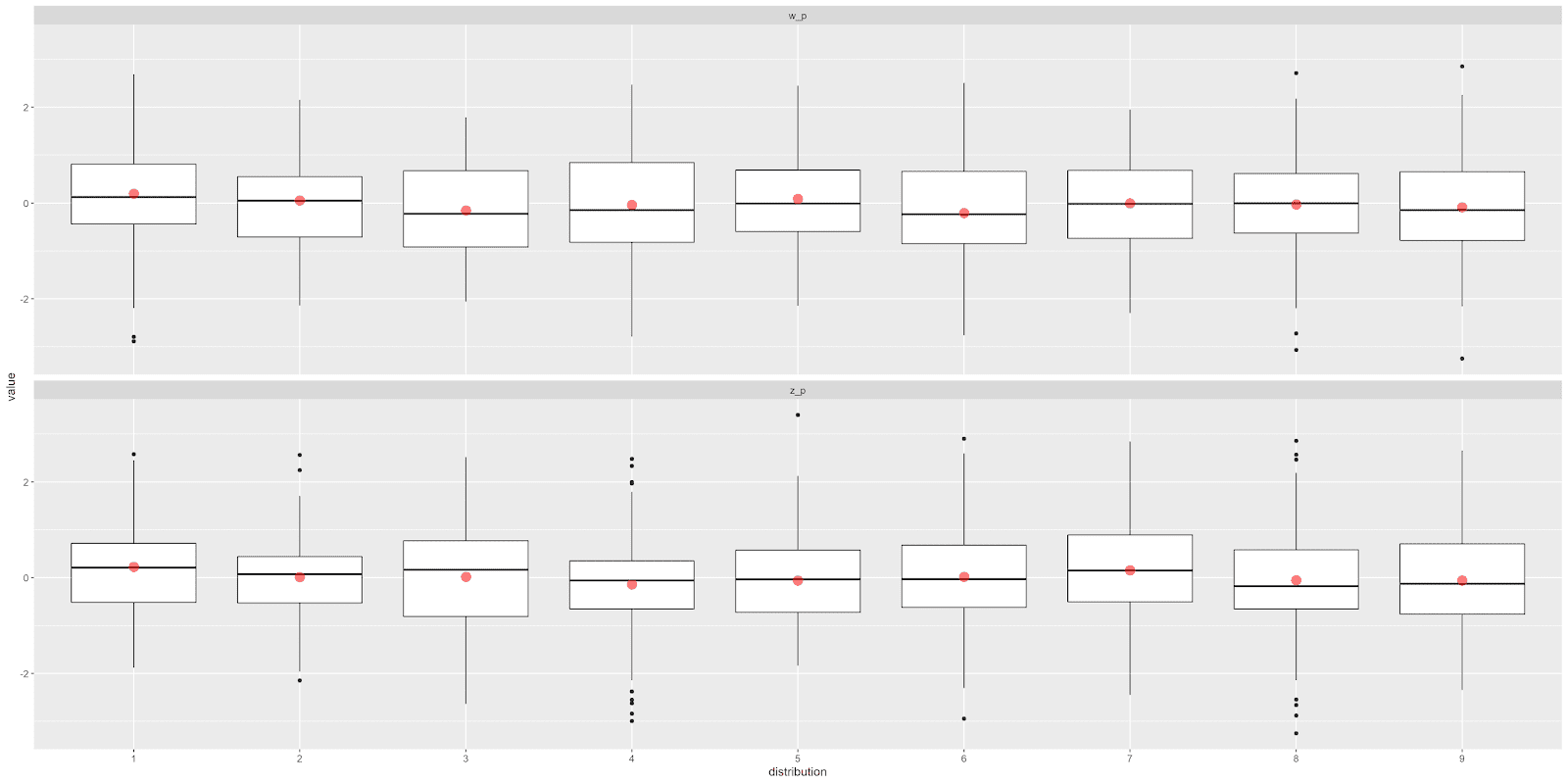
Now that the data is in tidy format, we can visualize both \(z'\) and \(w'\) with ggplot.

df %>%
    pivot_longer(
        names_to = "category", 
        values_to = "value", 
        cols = z_:w_
    ) %>% 
    ggplot(aes(x = distribution, y = value)) + 
    geom_boxplot() + 
    stat_summary(
        geom = "point", fun = mean, 
        size = 4, color = "red", alpha = 1/2
    ) +
    facet_wrap(~ category, nrow = 2)

The result is shown below: