Arithmetics concerning the recent urinatorium of post-MCO Malaysia
The recent example given in the BNM statement requires the use of a little bit of higher arithmetics, that is, in my opinion, beyond what the fictitious Makcik Kiah can readily verify and reproduce for other scenarios.

Fortunately she can probably consult his degree-holder son, a certain mister Liah, and ask him to verify BNM's calculations. The hire-purchase value in the simple-interest universe is quite easy to handle. The hire-purchase value for the \(n\)-th term is simply: $$p(n) = \underbrace{p_0}_{\rm base} + \underbrace{b_{\rm simple}n p_0}_{\rm interest} - \underbrace{n m}_{\rm deductions}$$ where \(t_{\rm simple} = 12 b_{\rm simple}\), \(m\) is the monthly instalment, \(n\) is the number of instalments, \(p_0\) is the initial hire-purchase value. Apparently Makcik Kiah can handle this calculation since it involves only the four basic arithmetic operations.
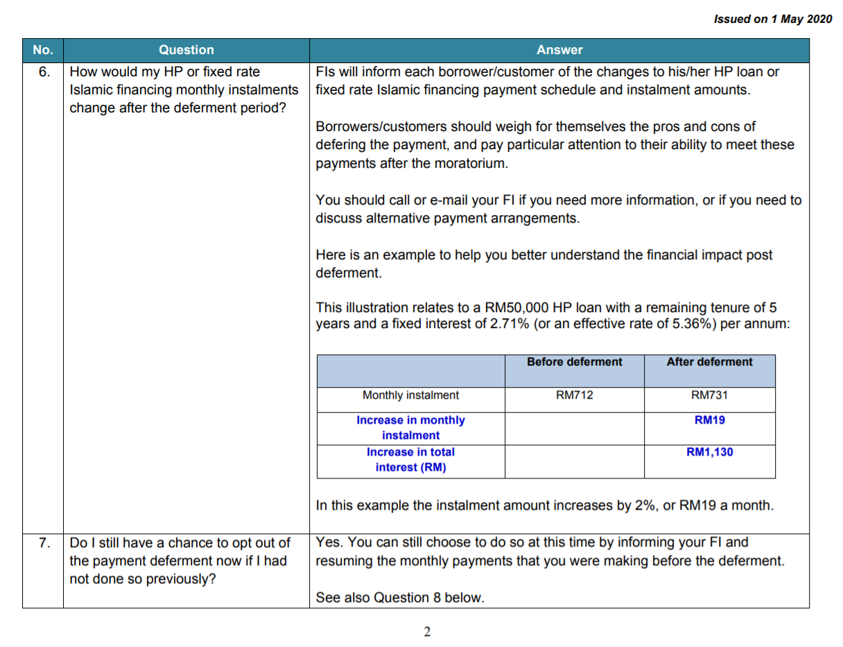
But the math is slightly more involved when the term effective interest is introduced. Thus as the first step, Liah reformulated the hire-purchase value time series in the compound-interest universe, which involves the following recurrence: $$p(n) = B[p(n-1) - m], \quad p(0) = p_0$$ where \(B\) is the bunga-factor given by \(B = 1 + b_{\rm effective}\) (\(b_{\rm interest}\) is the effective monthly bunga). He then proceeded to solve this recurrence equation, which resulted in: $$p(n) = \frac{m}{1-1/B} - B^n \left(\frac{m}{1-1/B} - p_0 \right)$$ Since \(p(0) = 0\), we must have \(m = p_0\left(\frac{1 - 1/B}{1 - 1/B^n}\right)\), which must then be set equal to the \(m\)-value in the simple interest universe. The equality can eventually be simplified to the following bullshit \(n\)-th order polynomial equation in \(B\) and \(S\): $$\left(\tfrac{1}{B}\right)^n - \tfrac{1}{S}\left(\tfrac{1}{B}\right) + (\tfrac{1}{S} -1) = 0$$ where \(S = b_{\rm simple} + \frac{1}{n}\). Liah learnt from his math class that the Frenchman Évariste Galois showed in 1831 that this equation which cannot be solved in closed form for \(n > 4\). Thus he used his Wolfram Alpha app to solve the case numerically for \(n = 84\) terms. The result is that the effective bulanan-interest is \(b_{\rm effective} = \frac{0.43268}{100}\), which is roughly a tahunan-interestLiah's result is slightly different from the value published by BNM. This is likely a result of the exact value of \(n\) used in the calculation. From \(m = 712\)-value given in BNM's example, Liah assumed a round number of contractual terms of \(n = 84\), but this is not specifically mentioned in the BNM example. The \(m\)-value in the BNM's example slightly odd because exact \(m\)-value obtained by applying the simple interest calculation ought to be 708.15 when \(n = 84\) and \(p_0 = 5\times 10^4\). If this number is round up to 709 as integer \(m\)-value for the first \(n-1\), then the last instalment is 638. Reversed calculation easily reveals that the \(n\)-value used in BNM's simulation could be \(n = 83\frac{1}{3}\) if one were to obtain \(m = 712\) exactly. of \(t_{\rm effective} = \frac{5.19}{100}\).
Liah then proceeded to apply the effective interest rate on the deferred amount. This part is a little tricky because Liah believes he has several options.
- Compounding method 1a. Zero interest during the six-month urinatorium period, but apply interest to the balance terms (but only up to the original contractual last terms). This way, the add-on can be calculated as: \begin{align} a_{\rm uri}^{\rm (1a)} &= 6m\left(B^{n_{\rm bal}-6} - 1\right)\\ &= 6p_0\left(\frac{t_{\rm simple}}{12} + \frac{1}{n}\right)\left(B^{n_{\rm bal}-6} - 1\right)\\ &= p_0 \lambda_{\rm 1a}(t_{\rm simple}, n, n_{\rm bal}, B(t_{\rm simple}, n)) \end{align}
- Compounding method 1b. Zero interest during the six-month urinatorium period, but apply interest to the balance terms (beyond the contractual last term to included the extended six terms). This way, the add-on can be calculated as: \begin{align} a_{\rm uri}^{\rm (1b)} &= 6m\left(B^{n_{\rm bal}} - 1\right)\\ &= 6p_0\left(\frac{t_{\rm simple}}{12} + \frac{1}{n}\right)\left(B^{n_{\rm bal}} - 1\right)\\ &= p_0 \lambda_{\rm 1b}(t_{\rm simple}, n, n_{\rm bal}, B(t_{\rm simple}, n)) \end{align}
- Compounding method 2. Apply interest to the balance terms up to the original contractual last term (including the 6 terms in urinatorium period). This way, the add-on can be calculated as: \begin{align} a_{\rm uri}^{(2)} &= m\left[\left(\frac{B^6-1}{B-1}\right)B^{n_{\rm bal}-6} - 6\right]\\ &= p_0\left(\frac{t_{\rm simple}}{12} + \frac{1}{n}\right)\left[\left(\frac{B^6-1}{B-1}\right)B^{n_{\rm bal}-6} - 6\right]\\ &= p_0 \lambda_2(t_{\rm simple}, n, n_{\rm bal}, B(t_{\rm simple}, n)) \end{align}
- Compounding method 3. The monthly instalments associated the original \((n_{\rm bal}-6)\) terms are not considered in calculation. A new reducing balance time series is constructed from the debt accumulated at the end of the urinatorium period. This way, the add-on can be calculated as: \begin{align} a_{\rm uri}^{(3)} = n_{\rm bal}m \left[\frac{6B^{n_{\rm bal}} - \left(\frac{B^{6}-1}{B-1}\right)}{B^6\left(\frac{B^{n_{\rm bal}-6}-1}{B-1}\right)+\left(\frac{B^6-1}{B-1}\right)}\right] \end{align}
| 0 | 1a | 1b | 2 | 3 | |
|---|---|---|---|---|---|
| Total add-on | \(0\) | \(1115.61\) | \(1256.39\) | \(1173.97\) | \(1062.47\) |
| Monthly spread-on | \(0\) | \(18.59\) | \(20.94\) | \(19.57\) | \(17.71\) |
| New normal | \(708.15\) | \(726.75\) | \(729.09\) | \(727.72\) | \(725.86\) |
Liah also took the figures in BNM's first numerical example and obtain the following numbers:
| 0 | 1a | 1b | 2 | 3 | |
|---|---|---|---|---|---|
| Total add-on | \(0\) | \(3358.87\) | \(3736.45\) | \(3515.08\) | \(2903.33\) |
| Monthly spread-on | \(0\) | \(46.65\) | \(51.90\) | \(48.82\) | \(40.32\) |
| New normal | \(1133.33\) | \(1179.98\) | \(1185.23\) | \(1182.15\) | \(1173.66\) |
Since \(\lambda\) is an exponential function of \(n_{\rm bal}\), Liah warned his mother not to over-generalize and re-apply the result of 2-percent increase in monthly-repayment to her sister Makcik Miah, since in Makcik Miah's case, she has only managed to clear 6 out of her 108 contractual terms. In Makcik Miah's case, the percentage increase is: $$ \lambda_2\left(\tfrac{3}{100}, 108, 102, 1 + \tfrac{0.468}{100}\right) \approx 4.1156\% $$ If Makcik Miah initial principal is \(200\times10^3\), this 4.1% add-on means an additional 10454 ringgit for the entire remaining tenure of 102 terms.


Comments