Rigel Kent

Suppose \((t, \dot{s}_{\ell}(t))\) is the time series of liquid sugar mass flow measurement in Line \(\ell\) of a certain factory. To compute the liquid sugar mass for a given interval \(t \in [t_{\rm start}, t_{\rm stop}]\), we can integrate the time series numerically: $$s(t_{\rm start}, t_{\rm stop}, \ell)=\int_{t_{\rm start}}^{t_{\rm stop}} \dot{s}_{\ell}(t)\,dt$$ For instance, the following line totalizes the liquid sugar flow in Line 1 between 11:00 am to 12:00 pm on June 29. sugar_mass('2020-6-29 11:00', '2020-6-29 12:00', 'L1_sugar_massflow') where sugar_mass is totalizer function which parse the mass flow time series into a numerical value. Suppose you are given the task to compute the total sugar metered by flowmeters in Lines 1, 2, 4, and 6 for that same interval. A quick and dirty way would be to rewrite the original code like this: start_clock A slightly better approach is to use start_clock where all_sugar is a reusable function...

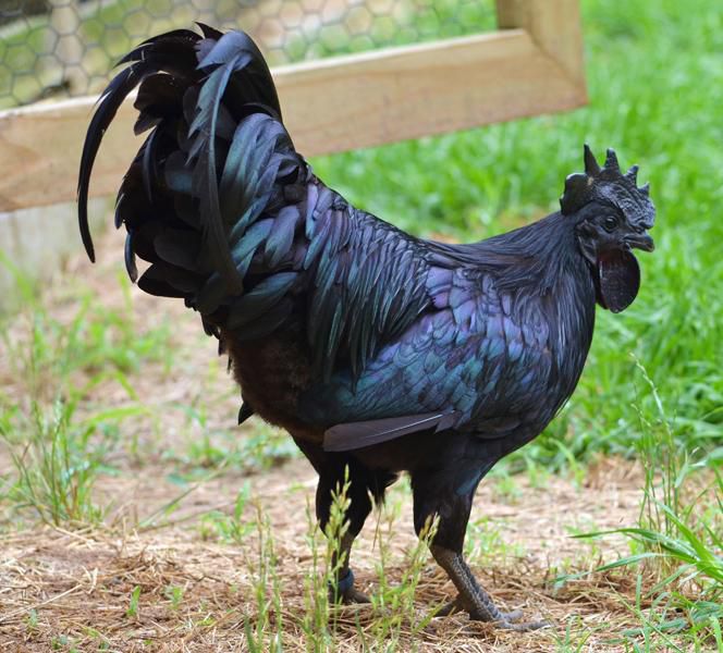
The following is the concluding conversation between Sun Wukong and Mañjuśrī Bodhisattva in Chapter 39 of The Journey to the West. This is also the story told in the first test episode of TV-adaptation of the novel (Episode name: Quelling the rākṣasa in the Kingdom of Kadaknath 除妖烏雞國) screened by CCTV in 1982. Black chickens are artificially selected for their black appearance. They can be found in many parts of the world and are known by different names: Cemani (Java), Kadakhnath or Kali masi (India), Black H’Mong (Vietnam), Argentinean Tuzo (Latin America), and Svarthöna (Sweden), Silkie (China). See Anik Budhi Dharmayanthi, Yohei Terai, Sri Sulandari, M. Syamsul Arifin Zein, Toyoko Akiyama, Yoko Satta (2017) The origin and evolution of fibromelanosis in domesticated chickens: Genomic comparison of Indonesian Cemani and Chinese Silkie breeds , PLOS ONE. The conversation started with Sun Wukong reprimanding Mañjuśrī bodhisattva for not able to control his subordinates. Wuk...

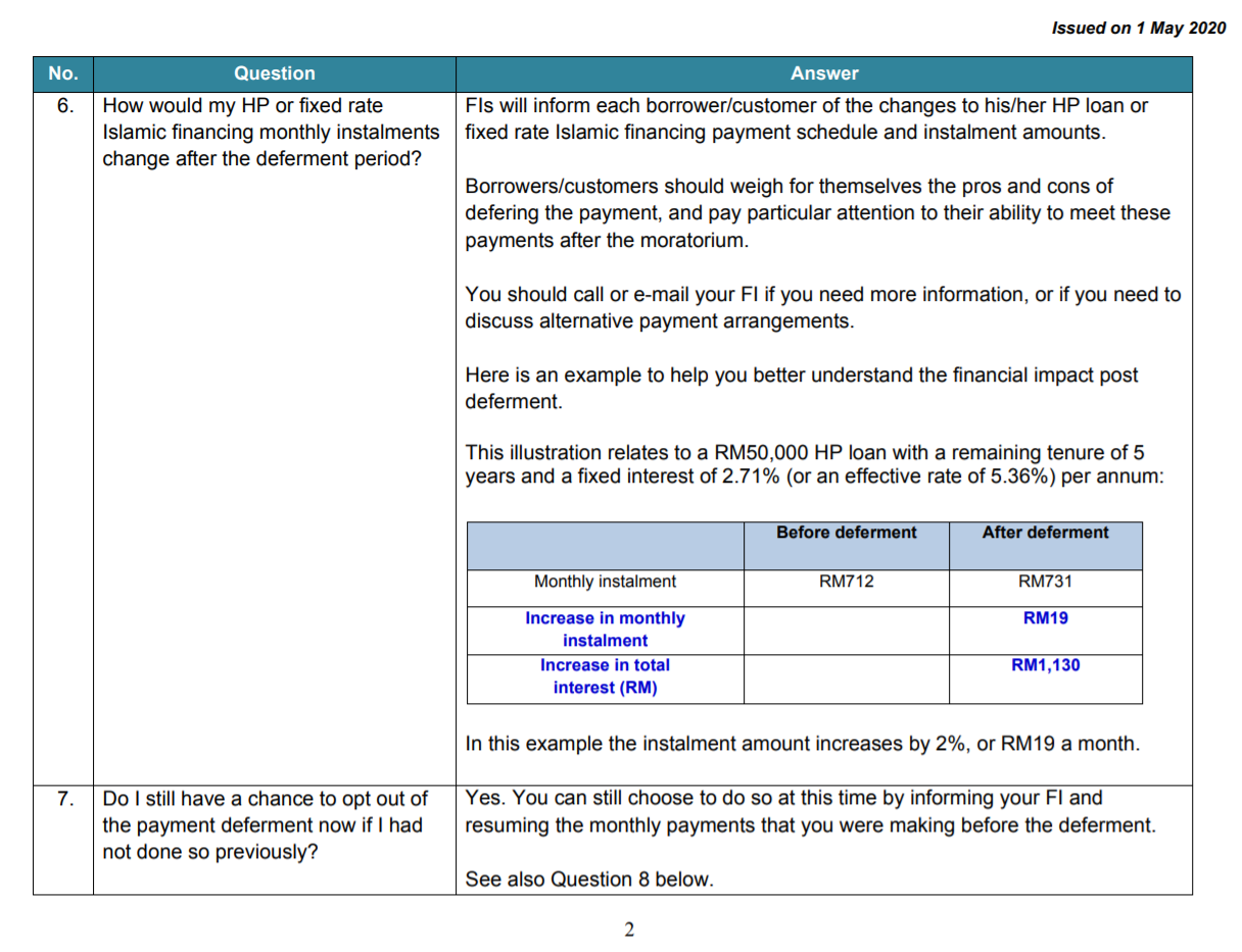
The recent example given in the BNM statement requires the use of a little bit of higher arithmetics, that is, in my opinion, beyond what the fictitious Makcik Kiah can readily verify and reproduce for other scenarios. Second numerical example issued by BNM on 1 May 2020. Apparently she was underwhelmed by new additional, albeit razor thin, 19-ringgit-add-on spread across her debt time series post-October, which is presented in stark contrast to the earlier 0-ringgit-add-on scenario exemplified In the first numerical example given by BNM, they used \(p_0 = 9\times 10^4\), \(n = 108\) terms, balance \(n_{\rm bal} = 72\) terms, \(p_0=1133\) on 27 March 2020. First numerical example issued by BNM on 27 March 2020. Fortunately she can probably consult his degree-holder son, a certain mister Liah, and ask him to verify BNM's calculations. The hire-purchase value in the simple-interest universe is quite easy to handle. The hire-purchase value for the \(n\)...

Around 1640 Fermat documented this method in a awkwardly titled paper: De aequationum localium transmutatione et emendatione ad multimodam curvilineorum inter se vel cum rectilineis comparationem (On the transformation and alteration of local equations for the purpose of variously comparing curvilinear figures among themselves or to rectilinear figures, to which is attached the use of geometric proportions in squaring an infinite number of parabolas and hyperbolas). The ideas presented in the paper was dated probably 20 years ago but it was only written in 1658, two years after the publication of John Wallis's Arithmetica Infinitorum (1656). But it was not published or circulated until 1679. , 30 years before Newton and Leibniz officially “invented" calculus, Fermat managed to convinced himself that $$\int_0^k x^n\,dx= \frac{k^{n+1}}{n+1} = L(n+1)$$ Fermat's trick was to slice the area under the curve of \(y = x^n\) into infinitely many irregular intervals so that the ...

In 1720, Christian Goldbach's experiments with infinite series was published in the German journal Acta Eruditorum , he titled his paper Specimen methodi ad summas serierum and proceeded to furnish a number of worked examples The following examples are given in Goldbach's 1720 paper: \begin{align}\tfrac{1}{2}+\tfrac{1}{6}+\tfrac{1}{12}+\tfrac{1}{20}+\ldots\\ \tfrac{2}{64}+\tfrac{11}{544}+\tfrac{26}{1972}+\tfrac{47}{5104}+\ldots \\ \tfrac{1}{2}+\tfrac{1}{4}+\tfrac{1}{8}+\tfrac{1}{16}+\ldots \\ \tfrac{1}{3}+\tfrac{1}{81}+\tfrac{1}{19683}+\tfrac{1}{43046721} + \ldots\end{align}whose general terms are \(\frac{1}{x^2+x}\), \(\frac{3x^2-1}{9x^4+36x^3+33x^2-6x-8}\), \(\frac{1}{2x}\), and \(\frac{1}{2x^x-x}\). of his finite difference technique for relocating the general term of a given sequence. The general principle is that in the general case, the \(n\)-th term, \(a_n\), of any number sequence $$a_1, a_2, a_3, \ldots$$ can be expressed by using an infinite series involving ...

Anybody with one-to-two years of basic calculus exposure can easily work out the following definite integral of \(x^n\): $$\int_{0}^k x^n \,dx = \frac{k^{n+1}}{n+1} = {\rm L}(n + 1)$$ where \({\rm L}(n) = {k^n}/{n}\). This is a mid-17th-century result known to both Newton and Leibniz , but their results were not written in modern notation In his 1669 paper “De Analysi per Aequationes Numero Terminorum Infinitas" (Of analysis by equations of an infinite number of terms), Newton wrote: Let the base \(AB\) of any curve \(AD\) have \(BD\) for its perpendicular ordinate; and call \(AB = x\), \(BD = y\), and let \(a, b, c,\) etc be given quantities, and \(m\) and \(n\) whole numbers, then following rule (Rule I) can be used to compute the quadrature of simple curves. If \(ax^{m/n}=y\), then$$\frac{an}{m+n}x^{\frac{m+n}{n}} = {\rm area} \, ABD$$Newton then proceeded to give a number of examples. He wrote: The thing will be evident by an example. If \(x^2 = y\), th...

General Mara Averick's blog . R for Data Science by Garrett Grolemund and Hadley Wickham. R for Data Science: Exercise Solutions by Jeffrey B. Arnold. Hands-On Programming with R by Garrett Grolemund. The Tidyverse Cookbook by Garrett Grolemund. Tidy Evaluation by Lionel Henry and Hadley Wickham. Functional Programming by Sara Altman, Bill Behrman, and Hadley Wickham. Advanced R by Hadley Wickham. Advanced R Solutions by Malte Grosser, Henning Bumann and Hadley Wickham. Make your R roar by Purrring by Gavin Fay. Geocomputation with R by Robin Lovelace, Jakub Nowosad, Jannes Muenchow. R Packages by Hadley Wickham and Jenny Bryan. R Cookbook by James Long and Paul Teetor. R语言忍者秘笈 by 谢益辉, 肖楠, 坑主三, and 坑主四. Stat405: Introduction to Data Analysis (Fall 2012, Rice University) by Hadley Wickham. Stat545: Data wrangling, exploration, and analysis with R by Jenny Bryan. Data Visualization ggplot2: Elegant Graphics for Data Analysis by Hadley Wic...

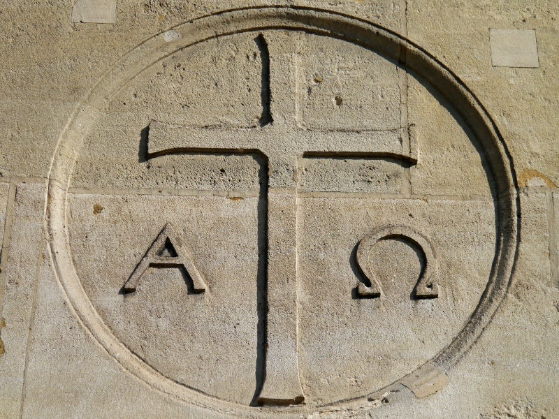
Euler's formula $$e^{i \Omega} = \sin \left(A- \Omega \right) + i \sin \Omega,$$ where \(A = \tfrac{1}{2}\pi\), is an interesting formula because we can use it express various types of sins in our complex world, and it says that sins of various degrees are ultimately imaginary. Here is the proof. First we suppose \(\Omega = \tfrac{1}{2}\pi \omega\), since $$e^{i\pi \omega/2} = e^{(i\pi/2)\omega}=\left(e^{i\pi/2}\right)^\omega $$we must have $$\sin \left(A - \tfrac{1}{2}\pi \omega \right) + i \sin \tfrac{1}{2}\pi \omega = \left[\sin \left(A - \tfrac{1}{2}\pi \right) + i \sin \tfrac{1}{2}\pi\right]^{\omega}=i^\omega$$ and if we start with \(\Omega = -\tfrac{1}{2}\pi \omega\), the following is true: $$\sin \left(A + \tfrac{1}{2}\pi \omega \right) - i \sin \tfrac{1}{2}\pi \omega = \left[\sin \left(A + \tfrac{1}{2}\pi \right) - i \sin \tfrac{1}{2}\pi\right]^{\omega} = (-i)^\omega$$ Since \(\sin \left(A+ \tfrac{1}{2}\pi \omega \right)=\sin \left(A - \tfrac{1}{2}\pi \omega \righ...

Suppose we have a function \(y = f(x)\) and its value at \(x = a\), \(f(a)\) is a nice value and can be easily calculated. Apparently, a slight perturbation on \(x\) from \(x = a\) to \(x = a + \epsilon\) will be accompanied by a slight change in the value of \(y\), where \(a \gg \epsilon\). Computation of the new value of \(y\), that is, \(f(a + \epsilon)\) is one of the standard operating procedure taught in the fourth-form calculus. For instance, in 2017, the following question appeared as the second question in the second paper of the SPM additional mathematics exam. It is given that the equation of a curve is \(y = \frac{5}{x^2}\). Find the value of \(\frac{{\rm d}y}{{\rm d}x}\) when \(y = 3\). Hence estimate the value of \(\frac{5}{2.98^2}.\) The standard textbook trick uses only the first two terms in the following series: $$f(a + \epsilon) = \sum_{k=0}^\infty \frac{f^{(k)}(a) \epsilon^k}{k!}$$ that is, $$f(a + \epsilon) \approx f(a) + f'(a) \epsilon$$ a...

The SIR (susceptible/infected/removed) model in epidemiology is first considered nearly 100 years ago by two Scottish doctors, William Kermark (1898-1970) and Anderson McKendrick (1876-1943) (see W. O. Kermack and A. G. McKendrick (1927) Contribution to the mathematical theory of epidemics , Proc. Roy. Soc. Lond A 115, 700-721). In 1927, they opened their paper with the following line: One of the most striking features in the study of epidemics is the difficulty of finding a causal factor which appears to be adequate to account for the magnitude of the frequent epidemics of disease which visit almost every population... When a group of infectious species, \(I\), is introduced into a community of susceptible species, \(S\) (which is not previously exposed to the RNA materials), the virus spreads from the infectious species to the susceptible species, thus diminishing the susceptible species and growing the size of the infectious species. $$I + S \longrightarrow I' + S'...

Cyril Northcote Parkinson (b. 1909, d. 1993) 是馬來亞大學的第一任萊佛士歷史教授。 他是第二任萊佛士歷史教授K. G. Tregonning (b. 1923, d. 2015) 的博士論文導師，而Tregonning後來是邱繼金 Khoo Kay Kim (b. 1937, d. 2019) 的學士論文導師。所以算起來，Parkinson是邱老師的師公。 By skipping over Tan Sri Khoo’s PhD supervisor, Eddin Khoo Bu Eng 邱武英 has helpfully demonstrated his unique scholarly method: if you don’t know something, simply pretend it never existed. A bold strategy, historically used by small children and certain governments. For anyone actually interested in Tan Sri Khoo’s academic journey — which, unlike Eddin’s version, involves real dates, real theses, and real supervisors — here it is: K. K. Khoo (1960) The municipal government of Singapore, 1887 - 1940, B. A. Thesis, Department of History, University of Malaya. Tan Sri was 23, which is around the age when most of us were still trying to figure out how library catalogues worked. K. K. Khoo (1967) The western Malay states, 1861 - 1873: The political effe...